

Introduction to R Shiny Reactivity with Hands-on Examples


 Share
Share Tweet
Tweet Share
ShareR Shiny is all about reactivity. It’s a paradigm that allows you to build responsive and interactive applications by implementing data-driven interfaces. Changes triggered by the user will be immediately reflected in the application. Long story short, master R Shiny reactivity and you’ll master Shiny.
But where do you start learning about reactivity in the R Shiny application? Well, reading this article might be a good idea. We’ll provide you with insights into what reactivity is, why it’s an essential concept in R Shiny, what are reactive inputs, expressions, and outputs, and much more. Let’s dig in!
R Programming and R Shiny can improve your business workflows – Here are 5 ways how.
Table of contents:
- Introduction to Reactivity and its Importance in R Shiny Apps
- Basic Reactivity in R Shiny
- R Shiny Reactivity with Reactive Inputs
- Reactive Expressions – Everything You Need to Know
- Reactive Outputs in R Shiny
- Summing up R Shiny Reactivity
Introduction to Reactivity and its Importance in R Shiny Apps
So, the big question is – What is reactivity in the context of R Shiny? Well, it refers to the concept of powering the interactivity and responsiveness of Shiny applications. It means that everything you interact with, such as dropdowns and buttons, will automatically trigger a change in the user interface. It happens behind the scenes, and you don’t have to wait for the page to reload.
Here are a couple of fundamental principles on which R Shiny reactivity is based upon:
- Reactive inputs: Input elements of an R Shiny app, such as text inputs, checkboxes, dropdowns, sliders, and so on. When a user interacts with these inputs, they generate reactive values.
- Reactive outputs: Components of an R Shiny application that display the results of reactive expressions. Think of these as charts, tables, or anything else that can be updated based on the change in reactive expressions or inputs.
- Reactive expressions: R expressions that take reactive inputs as inputs. They are used to perform calculations, transformations, or any sort of data manipulation.
R Shiny will automatically detect which reactive expression depends on which input, and also automatically make changes when needed.
Let’s now see how R Shiny reactivity works in practice by going over reactive inputs.
R Shiny Reactivity with Reactive Inputs
In R Shiny, reactive inputs and outputs are closely tied together. It’s challenging to talk about one without mentioning the other, so expect to see some reactive outputs in this section as well. It’s needed to render the results of reactive inputs.
Don’t worry, we’ll still cover reactive outputs in much more depth later in the article.
Example 1: Handling Simple Input
Let’s get straight to business. R Shiny provides a ton of functions that end with Input(), such as textInput() or numericInput(). You can use these to create input elements and pass in adequate properties.
The example you’ll see below declares one textual and one numeric input, gives them IDs, labels, and default values, and also declares an output element for rendering the input values. Don’t worry about the output portion – we’ll cover it later in the article. For now, try to understand the input elements, and just copy/paste the output portion.
The server() function of an R Shiny application is where the magic happens. Long story short, that’s where you connect your inputs and outputs, and that’s also where you can access the input values. Our example will only leverage the paste() function to display a simple message that depends on the current value of the input elements:
library(shiny)


ui <- fluidPage(
  # Note the inputId property
  textInput(inputId = "inName", label = "Your name:", value = "Bob"),
  numericInput(inputId = "inAge", label = "Your age:", value = 20),
  tags$hr(),
  # Note the outputId property
  textOutput(outputId = "outResult")
)


server <- function(input, output) {
  # This is how we access output elements
  output$outResult <- renderText({
    # This is how we access input elements
    paste(input$inName, "is", input$inAge, "years old.")
  })
}


shinyApp(ui = ui, server = server)
Here’s what you’ll see when you run the Shiny application:
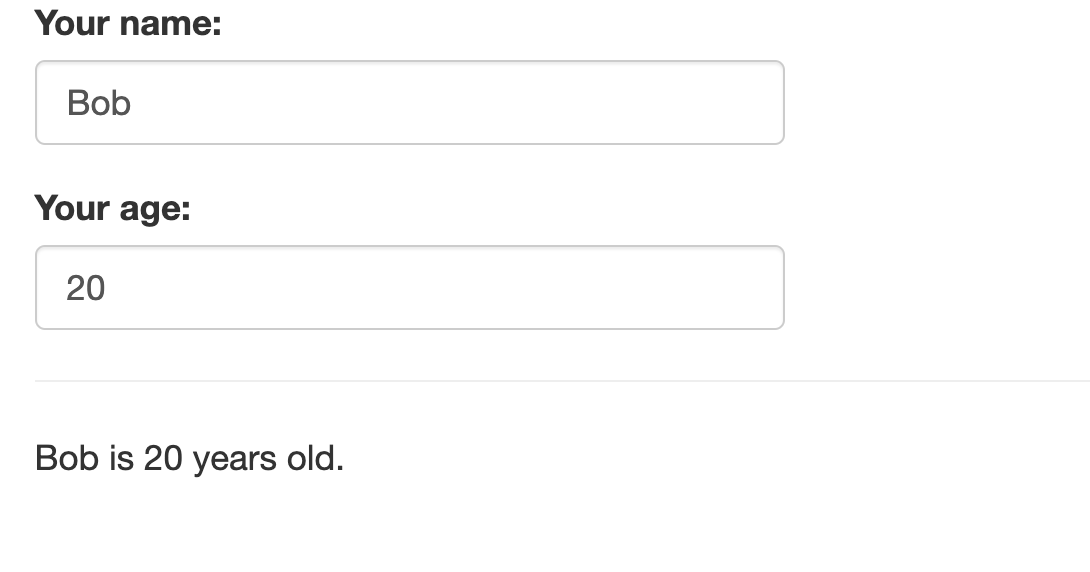
Image 1 – Simple input example 1
As you would assume, the output message changes automatically as soon as you change one of the inputs:
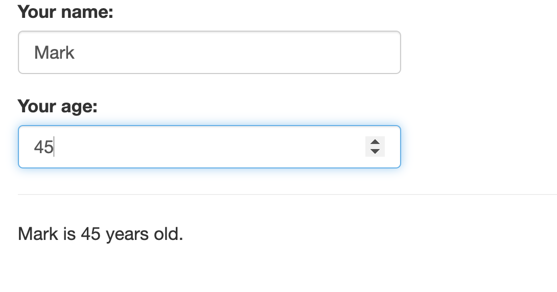
Image 2 – Simple input example 2
And that’s basic reactivity for you. Let’s take a look at a more detailed example next.
Example 2: Handling UI Elements
This example will show you how to leverage some additional input elements built into R Shiny. To be more precise, you’ll learn how to work with dropdowns, sliders, and checkboxes. We’ll tie everything into a simple employee evaluation example.
You can add dropdowns, sliders, and checkboxes to your R Shiny app by using the built-in selectInput(), sliderInput(), and checkboxInput() functions. Keep in mind that each requires a different set of parameters. For example, the selectInput() function needs an array of values and the default value, while the sliderInput() needs the range of values (min and max).
Inside the server() function, we’ll once again use the paste() function to combine multiple strings. There’s also an additional conditional statement, just to provide a better format for the output string. As before, don’t worry about the renderText() reactive function:
library(shiny)


ui <- fluidPage(
  textInput(inputId = "inText", label = "Enter name:"),
  selectInput(inputId = "inSelect", label = "Select department:", choices = c("IT", "Sales", "Marketing"), selected = "IT"),
  sliderInput(inputId = "inSlider", label = "Years of experience:", min = 1, max = 20, value = 5),
  checkboxInput(inputId = "inCbx", label = "Has R Shiny experience?"),
  tags$hr(),
  textOutput(outputId = "outResult")
)


server <- function(input, output) {
  # Determine different string value based on the checkbox
  output$outResult <- renderText({
    text_addition <- ""

    if (input$inCbx) {
      text_addition <- "has"
    } else {
      text_addition <- "has no"
    }

    paste(input$inText, "has worked in", input$inSelect, "department for", input$inSlider, "years and", text_addition, "experience in R Shiny.")
  })
}


shinyApp(ui = ui, server = server)
Here’s what you’ll see when you run the app:
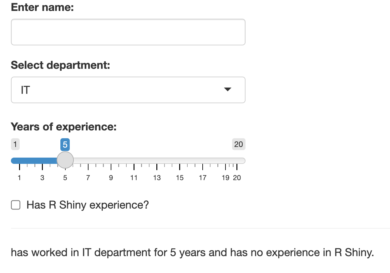
Image 3 – UI elements example 1
Note how the inText input doesn’t have a default value, so nothing is shown. As before, you can change any of the inputs and the output string will reflect these changes automatically:


Image 4 – UI elements example 2
And finally, let’s also tackle an essential R data structure – Data Frame.
Example 3: Handling Data Frames
Data Frames are everywhere in R, and you’re almost guaranteed to work with them when building a Shiny application. Think of them as of Excel spreadsheets, since they contain data organized into rows and columns.
We’ll keep the example fairly simple, and have a Data Frame with three columns. Users can select which one is displayed on the Y axis, and the chart is updated automatically upon change. To keep things even more simple, we’ll use R’s ggplot2 for displaying data visualizations:
library(shiny)
library(ggplot2)

# Dummy data.frame
data <- data.frame(
  X = 1:10,
  Y1 = 1:10,
  Y2 = 10:1
)

ui <- fluidPage(
  selectInput(inputId = "inY", label = "Y column:", choices = c("Y1", "Y2"), selected = "Y1"),
  plotOutput(outputId = "outChart")
)

server <- function(input, output) {
  output$outChart <- renderPlot({
    # Get the selected column
    selected_col <- input$inY
    # Render the chart
    ggplot(data, aes_string(x = "X", y = selected_col)) +
      geom_point() +
      labs(title = "Scatter plot")
  })
}


shinyApp(ui = ui, server = server)
This is what the app looks like when you first open it:


Image 5 – Chart example 1
And as before, the output element is updated automatically when a change in input is detected:

Image 6 – Chart example 2
Do you need more assistance in understanding ggplot2 code? We have plenty of articles for you, covering bar charts, line charts, scatter plots, box plots, and histograms.
And that’s it for a basic introduction to reactive inputs. Up next, we’ll go over reactive expressions.
Reactive Expressions – Everything You Need to Know
There are two functions you must know about when learning reactive expressions – reactive() and observe(). The prior is used to create reactive expressions from a block of R code – as simple as that. What’s neat about it is that you can reuse the result in multiple places. The latter is used to create a reactive observer, which is a piece of code that runs every time one of the inputs changes. It yields no output and can’t be used as an input to other reactive expressions.
Want to learn more about the Reactive observer in R Shiny? We have a full dedicated article on the topic.
Let’s now go over a couple of examples demonstrating reactive expression in R Shiny.
Example 1: Basic Reactive Calculation
This first example if probably the easiest one you’ll see. Ever! It simply takes two inputs, sums them, and stores the result inside a reactive expression.
Note how the reactive expression is stored inside a set of curly brackets – this indicates it’s an expression.
Also, always remember to call the reactive expression when you want to access its value. Think of this as calling a function. It’s not the same in theory, but the implementation is identical.
Anyhow, here’s the full code snippet for this basic example:
library(shiny)

ui <- fluidPage(
  numericInput("num1", "Number 1:", value = 3),
  numericInput("num2", "Number 2:", value = 5),
  tags$hr(),
  textOutput("sum")
)

server <- function(input, output) {
  # Calculate the sum and store it as a reactive expression
  sum_result <- reactive({
    input$num1 + input$num2
  })

  # Output to display the sum
  output$sum <- renderText({
    paste("Sum:", sum_result())
  })
}

shinyApp(ui = ui, server = server)
You’ll see the two input numbers summed and rendered when you first launch the app:
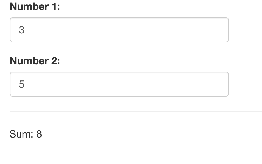
Image 7 – Simple reactive calculation example 1
As before, you can change the input elements and the output will re-render automatically:
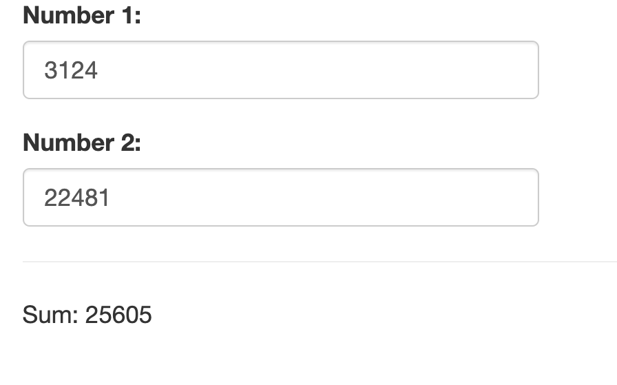
Image 8 – Simple reactive calculation example 2
And that’s a basic reactive expression for you. Up next, let’s see how to implement a reactive observer.
Example 2: Factorial Calculation and Reactive Observer
As briefly mentioned at the beginning of this section, a reactive observer is a simple piece of code that runs every time one of the inputs changes. They are only useful for their “side effects”, such as I/O, triggering a pop-up, and so on.
In this example, we’ll use a reactive observer to log a message to the console as soon as the numeric input changes. Further, we’ll use this numeric input to calculate and display a factorial of it.
Here’s the full code snippet for both the reactive expression and reactive observer:
library(shiny)

ui <- fluidPage(
  numericInput("num", "Enter a number:", value = 3),
  verbatimTextOutput("factorial")
)

server <- function(input, output) {
  # Calculate the factorial and store it as a reactive expression
  factorial_result <- reactive({
    n <- input$num
    if (n == 0) {
      return(1)
    } else {
      return(prod(1:n))
    }
  })

  # Runs every time the input changes
  observe({
    n <- input$num
    cat("Calculating factorial of", n, "\n")
  })

  # Display the factorial
  output$factorial <- renderPrint({
    factorial_result()
  })
}

shinyApp(ui, server)
Launching the app will display the input number and its factorial:
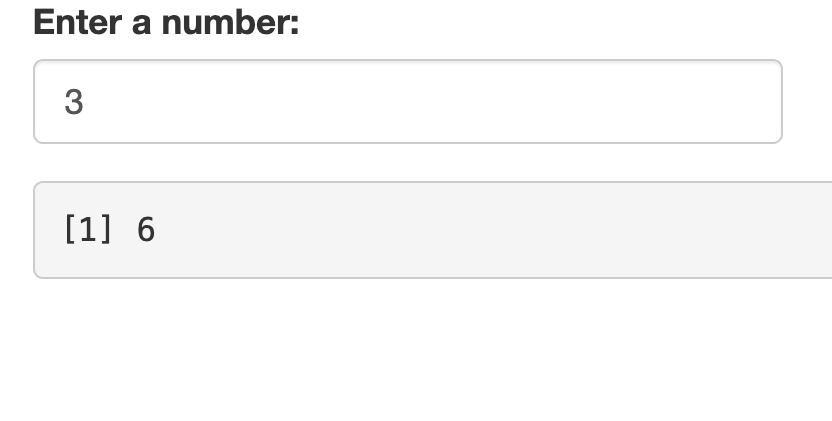
Image 9 – Reactive observer example 1
You can change the input value, and the output is re-rendered instantly:
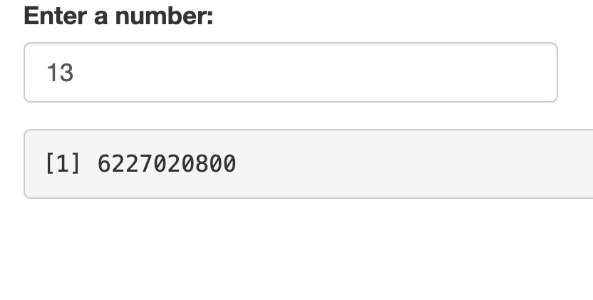
Image 10 – Reactive observer example 2
The reactive observer logs our message to the R console. You’ll see it in the Console tab of RStudio:
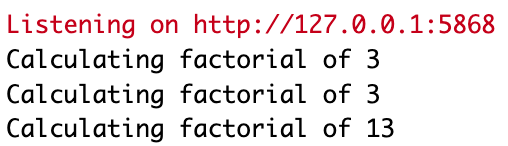
Image 11 – Reactive observer console output
Simple, right? Let’s go over one more example.
Example 3: Filtering Data Frames
You’ve seen in the previous section that Data Frames are everywhere. Data science revolves around data, and data frames provide a convenient data structure for data storage and manipulation. It’s essential for you to know how to manipulate data, and this example will show you how to select multiple columns that are displayed in table form to the user.
We’ll use the built-in mtcars dataset to keep the code short and tidy. The filtered data will be stored in a filtered_data reactive expression, which further uses the req() function to ensure that at least one column is selected before filtering the data:
library(shiny)

ui <- fluidPage(
  selectInput(inputId = "cols", label = "Columns to display:", choices = names(mtcars), selected = c("mpg"), multiple = TRUE),
  tableOutput(outputId = "table")
)

server <- function(input, output) {
  # Filter the dataset based on selected columns and store it as a reactive expression
  filtered_data <- reactive({
    req(input$cols)
    selected_cols <- input$cols
    mtcars[, selected_cols, drop = FALSE]
  })

  # Display the output as a table
  output$table <- renderTable({
    filtered_data()
  })
}

shinyApp(ui, server)
As you can see, a single column is selected by default when you launch the app:


Image 12 – Data Frame filtering example 1
Since this is a multi-select dropdown menu, you can choose however many columns you want, and they’ll be added to the output table immediately:

Image 13 – Data Frame filtering example 2
These three examples will be enough to get your feet wet when it comes to reactive expressions.
Reactive Outputs in R Shiny
Truth be told, this is the section in which you’ll learn the least. Not because there’s not much to learn, but because we’ve been working with reactive outputs through the entire article. It’s near impossible to demonstrate what reactive inputs and expressions do if you don’t display their results – and that’s where the output comes in.
Still, we’ll provide you with a couple of useful and practical examples. We’ll also dive a bit deeper into how reactive outputs are structured.
Every reactive output function begins with render, such as renderText(), renderPlot(), and so on. There are many built-in rendering functions, but some R packages will also bring their own. You’ll see two such examples later in this section.
But first, let’s start with the basics.
Example 1: Rendering Text
If you’ve gone through the first section of this article, this example will feel like a recap. The idea is to allow the user to enter a number and then to render that number as a textual message. Simple!
R Shiny uses the textOutput() function as a container for the textual output element. Inside the server function, you’ll have to call the renderText() function and pass in the expression.
And that’s the general pattern – xOutput() function in the UI followed by renderX() function in the server. Something to keep in mind.
Anyhow, here’s the full code snippet:
library(shiny)

ui <- fluidPage(
  numericInput(inputId = "num", label = "Enter a number:", value = 5),
  tags$hr(),
  textOutput(outputId = "text")
)

server <- function(input, output) {
  # Use the renderText() reactive function in combination with textOutput()
  output$text <- renderText({
    input_num <- input$num
    paste("You've entered:", input_num)
  })
}

shinyApp(ui = ui, server = server)
You’ve already seen a bunch of interesting examples, so this one will look a bit dull:
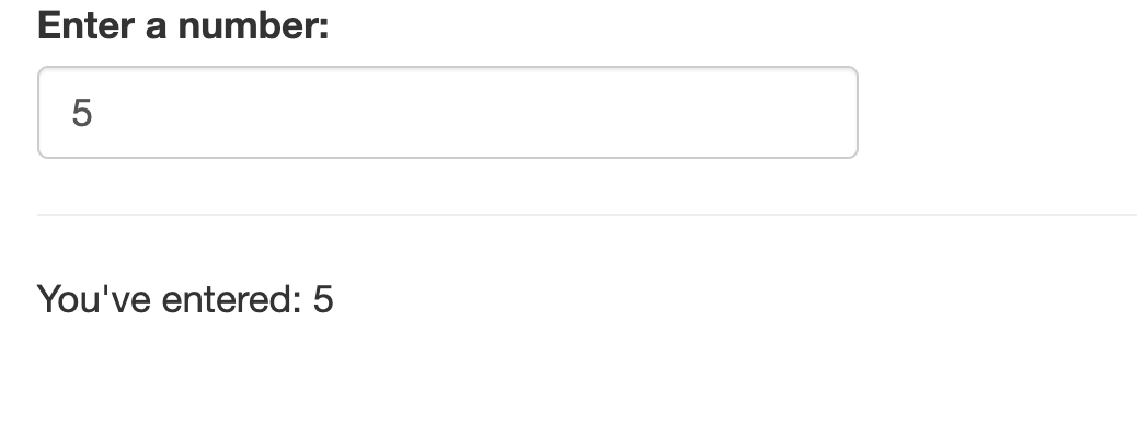
Image 14 – Text output example 1
As expected, the output message changes as you change the input:
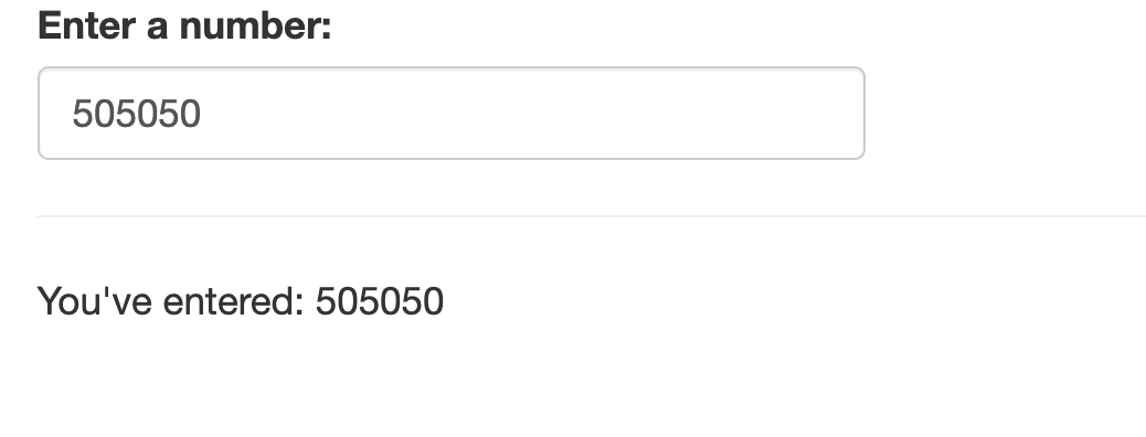
Image 15 – Text output example 2
Let’s now go over a much more interesting reactive output example.
Example 2: Rendering Interactive Charts
You’re not limited to using Shiny’s built-in output functions. Some external packages, such as Plotly, have their own set. This example will show you how to render an interactive Plotly scatter plot.
To be more precise, the app will allow the user to control the number of data points and the amount of noise, and will then combine the plotlyOutput() and renderPlotly() functions to produce the chart. The rest of the code is simple R and R Shiny logic:
library(shiny)
library(plotly)

ui <- fluidPage(
  sliderInput(inputId = "inPoints", label = "Number of Points:", min = 10, max = 100, value = 50),
  sliderInput(inputId = "inNoise", label = "Noise Level:", min = 0, max = 1, value = 0.2, step = 0.1),
  tags$hr(),
  # Note how it's plotlyOutput()
  plotlyOutput(outputId = "plot")
)

server <- function(input, output) {
  # Plotly has it's own reactive function
  output$plot <- renderPlotly({
    points <- input$inPoints
    noise <- input$inNoise

    set.seed(42)
    x <- 1:points
    y <- x + rnorm(points, sd = noise)

    plot_data <- data.frame(x = x, y = y)

    plot_ly(plot_data,
      x = ~x, y = ~y, type = "scatter", mode = "markers",
      marker = list(size = 10), text = ~ paste("X:", x, "
Y:", y)
    ) %>%
      layout(
        title = "Scatter Plot",
        xaxis = list(title = "X"),
        yaxis = list(title = "Y")
      )
  })
}

shinyApp(ui, server)
This is what the app will look like when you first launch it:
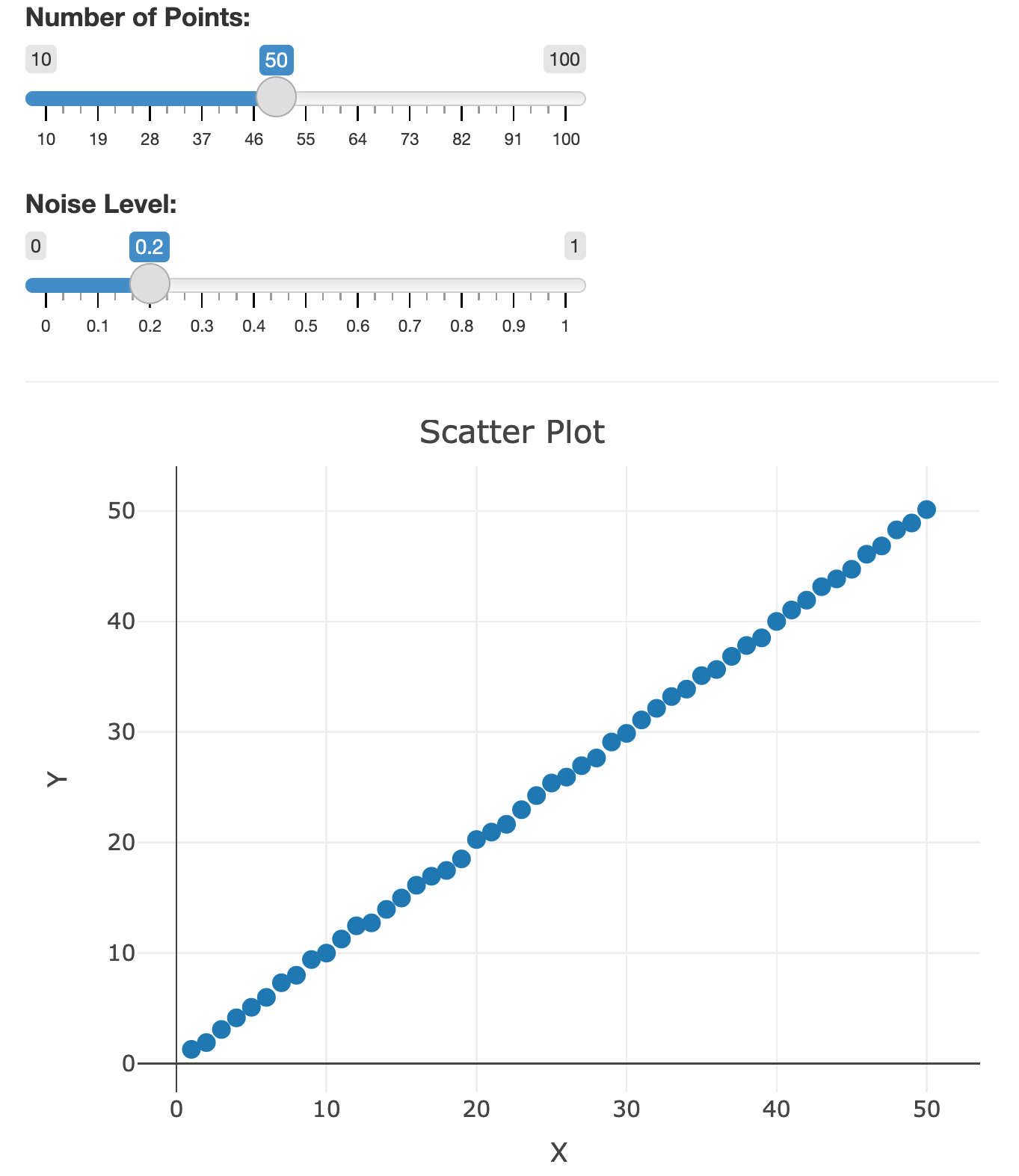
Image 16 – Plotly output example 1
Since Plotly is interactive, you can hover over individual data points to get more information:
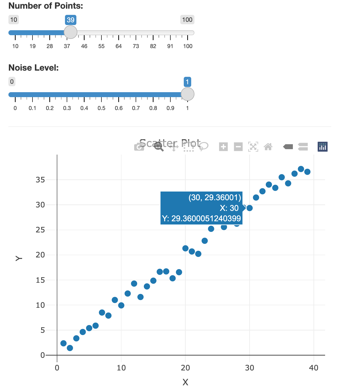
Image 17 – Plotly output example 1
You can see how an interactive R Shiny dashboard combined with an interactive charting library brings the best of both worlds.
Example 3: Rendering Data Tables
And finally, let’s look at yet another specialized R package for rendering data tables. It’s called DT and like Plotly, it brings its own set of functions – DTOutput() and renderDT().
We’ll use both to create a simple application that allows the user to control how many rows and columns are shown in a table. The actual cell values are arbitrary, and you shouldn’t look much into them.
Here’s the entire code snippet:
library(shiny)
library(DT)

ui <- fluidPage(
  sliderInput(inputId = "inRows", label = "Number of Rows:", min = 5, max = 20, value = 5),
  sliderInput(inputId = "inCols", label = "Number of Columns:", min = 2, max = 10, value = 2),
  # Note the specific DTOutput() function
  DTOutput(outputId = "table")
)

server <- function(input, output) {
  # DT has its own render function
  output$table <- renderDT({
    rows <- input$inRows
    cols <- input$inCols

    data <- matrix(runif(rows * cols), nrow = rows, ncol = cols)
    datatable(data)
  })
}

shinyApp(ui, server)
When launched, Shiny will show a data table with 5 rows and 2 columns:


Image 18 – DT output example 1
But you can easily change that by manipulating the slider values:


Image 19 – DT output example 1
The DT package is smart enough to not overflow the Shiny dashboard with too many rows. Instead, the table contents are paginated, which is one less thing for you to implement manually.
DT is not the only R package for rendering table Data – Here’s a bunch more you can try in R and R Shiny.
Summing up R Shiny Reactivity
For a core concept, R Shiny reactivity is utterly simple. Sure, it takes some time to get used to the syntax and the paradigm, but there’s not much to it in reality. It’s just a matter of practice and thinking ahead when planning an R Shiny project. Getting a good share of practice with reactive inputs, expressions, and outputs is all you need to make amazing Shiny apps.
Where things get interesting is when you want to build your own reactive components. That’s something we’ll go over in the following article, so make sure to stay tuned to the Appsilon blog.
Have a question about reactivity or need help on your enterprise Shiny project? Leave it to the experts – Make sure to drop us a message.
How does R Shiny handle state and what can you do when state is empty? shiny.emptystate comes to the rescue!
Contact Us
